Apollo Lander

Fly the Apollo 11 descent in a software-in-the-loop Monte Carlo campaign, then calibrate it against real telemetry.

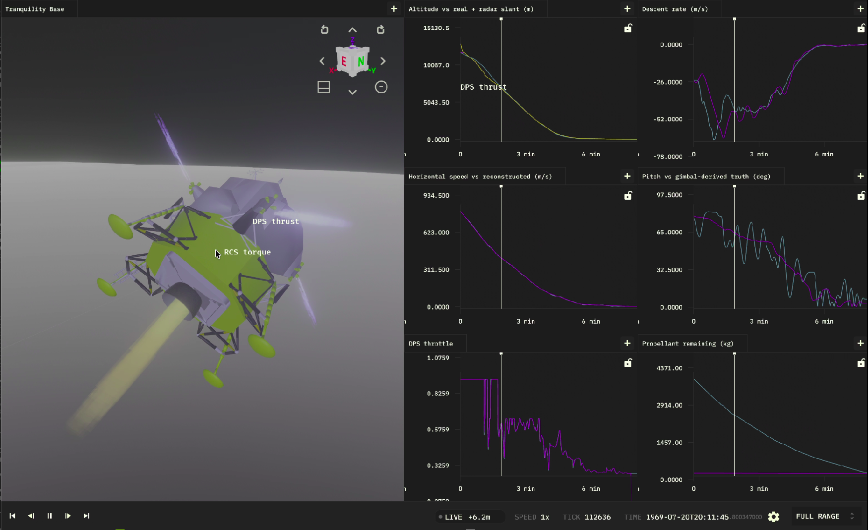
The bouncing-ball and three-body tutorials build a simulation and watch it run. Real aerospace work asks a harder question: does my actual flight software land the vehicle, across every dispersion it might see on the day? This tutorial answers it with the examples/apollo-lander example, which picks up Apollo 11 at landing-radar lock-on (~12 km up, still carrying ~800 m/s of orbital velocity) and flies the braking burn, pitchover, and touchdown with an external Lunar Guidance Computer (LGC) in the loop.

In this tutorial you'll learn to:

• Declare a simulation's tunable parameters for Monte Carlo
• Run ordinary Python in a post_step callback to drive a live flight-software process over a socket (software-in-the-loop)
• Launch and manage that process per run, with each parallel worker isolated
• Run a Monte Carlo campaign, score each run, and read an aggregated report
• Calibrate the model against real telemetry by narrowing parameter ranges

Rather than re-typing the whole example, we'll tour its key pieces and run them.

The big picture

A Monte Carlo SITL campaign has three moving parts:

• The simulation (sim.py): a 6-DOF lunar lander whose physics — gravity, the descent engine, RCS attitude control, and propellant burn-down — runs as JAX systems. It also replays the real Apollo descent on a "truth ghost" so you can compare against it.
• The flight software (controller/): a small Rust LGC that receives telemetry and sends back throttle and attitude commands, exactly like the real guidance computer. The simulation talks to it over UDP.
• The campaign runner (elodin monte-carlo): it samples a set of parameters, then fans the runs out across parallel workers. Each worker runs one descent — its own sim, its own controller, its own ports — and a pair of hooks score the runs and write a report.

spec.toml ──sample──▶ runner ──┬─▶ worker 1: sim ◀──UDP──▶ LGC ─┐
                               ├─▶ worker 2: sim ◀──UDP──▶ LGC ─┤─▶ score.py ─▶ report.py
                               └─▶ worker N: sim ◀──UDP──▶ LGC ─┘

Run it first

Clone the repo and launch the campaign from the repository root:

git clone https://github.com/elodin-sys/elodin.git && cd elodin

elodin monte-carlo run examples/apollo-lander/main.py \
  --campaign examples/apollo-lander/campaign.toml \
  --spec examples/apollo-lander/spec.toml \
  --out dbs/apollo-lander-demo

The runner builds the Rust controller once, samples 30 descents, and runs them in parallel (a few minutes on a laptop). When it finishes, it prints — and writes to dbs/apollo-lander-demo/post_campaign/apollo_lander_report.txt — a summary like:

Apollo 11 lander Monte Carlo report
====================================

runs completed: 30/30
soft landings: 27/30
success rate: 90.000%

Vertical touchdown speed
  mean: 1.471 m/s
  p95:  2.640 m/s
  max:  2.880 m/s

Landing dispersion (downrange miss from site)
  mean: 38.512 m
  p95:  94.000 m
  max:  121.880 m

Apollo telemetry fit
  best run: run-00017
  best altitude RMSE: 41.220 m
  mean pitch RMSE: 9.840 deg
  ...

Calibration hint
  Narrow spec.toml ranges around the best-fit params and re-run, or use
  calibrate.py for the optional automated loop.

Your exact numbers will vary, but you now have a working SITL campaign. The rest of the tutorial explains how each piece produced that report.

A guided tour of the pieces

Declare tunable parameters

A Monte Carlo campaign varies parameters. The simulation declares the ones it exposes with el.monte_carlo.params_spec(...) — each Param has a default and, optionally, a min/max range (sim.py, abbreviated to 3 of its 17):

PARAMS = el.monte_carlo.params_spec(
    init_altitude_m=el.monte_carlo.Param(float, default=11_800.0, min=11_650.0, max=11_950.0),
    init_pitch_deg=el.monte_carlo.Param(float, default=-77.0, min=-80.0, max=-70.0),
    propellant_kg=el.monte_carlo.Param(float, default=3_950.0, min=3_800.0, max=4_200.0),
    # ... 14 more: masses, gains, thrust scale, gravity, Isp ...
)

At runtime the sim reads the current row of sampled values with one call:

params = el.monte_carlo.params(PARAMS)
init_altitude = float(params.get("init_altitude_m"))

The simulation, in brief

sim.py exposes a build(params) function that returns (world, system): a 6-DOF lander with lunar gravity, a throttleable descent engine, RCS torque, and a mass-burn system, plus a kinematic truth ghost that replays the recorded Apollo descent every tick. Authoring physics systems is covered in the Bouncing Ball and Three-Body tutorials, so we won't dwell on it here.

The important distinction for SITL is this: the deterministic physics runs as JAX systems, but everything that talks to the outside world happens in a post_step callback — plain Python that runs after each tick.

Run real Python every tick: post_step and StepContext

world.run(..., post_step=fn) calls your function after each simulation tick (and pre_step=fn before it). Your callback receives the tick number and a StepContext, which gives you direct read/write access to the simulation database. Crucially, this is normal Python, not JAX — so you can open sockets, call libraries, and manage state across ticks.

The Apollo example uses exactly this to drive the live controller (main.py, abbreviated):

def post_step(tick: int, ctx: el.StepContext) -> None:
    # Read the latest kinematics straight from the simulation database.
    reads = ctx.component_batch_operation(
        reads=["lander.world_pos", "lander.world_vel", "lander.altitude",
               "lander.vertical_speed", "lander.propellant"]
    )
    altitude = float(reads["lander.altitude"][0])
    # ... assemble `state` from the readings and the reference profile ...

    # Ordinary Python: open the UDP socket once, then trade packets with the
    # live flight-software process.
    global bridge
    if bridge is None:
        bridge = SitlBridge(last_throttle, last_attitude)
    last_throttle, last_attitude, _ = bridge.step(state)

    # Write the commands back into the sim.
    ctx.component_batch_operation(
        writes={
            "lander.throttle_cmd": np.array([last_throttle]),
            "lander.attitude_setpoint": np.array(last_attitude),
        }
    )

StepContext also offers single-component read_component / write_component and the current ctx.tick / ctx.timestamp; component_batch_operation just does many reads and writes under one database lock.

But how do externally-written commands survive the next physics tick? The components the controller drives are tagged as externally controlled (sim.py):

ThrottleCmd = ty.Annotated[
    jax.Array,
    el.Component("throttle_cmd", el.ComponentType(el.PrimitiveType.F64, (1,)),
                 metadata={"external_control": "true"}),
]

Why software-in-the-loop?

You could approximate the guidance law inside a JAX system. SITL does something more valuable: it flies your actual flight software — the same code that will run on the vehicle — so the campaign exercises the real guidance and control logic, its real timing and lockstep behavior, and the simulation-to-software integration boundary, across every Monte Carlo dispersion. Bugs that only appear in the real code — numerical edge cases, message framing, off-by-one timing — surface here, in simulation, before they reach hardware.

Ways to connect your flight software

The post_step bridge is one option of several. Pick based on where your software runs:

• In-process bridge via post_step / pre_step + StepContext (sockets or IPC you open yourself) — what this example does. Lockstep, lowest latency, same process.
• A managed external process via world.recipe(...) — Elodin launches and tears down the real flight-software binary alongside the sim (covered next).
• A networked client over the Impeller2 protocol talking to elodin-db: any external program — or hardware-in-the-loop rig — reads sensor components and writes external_control commands without an in-process bridge.

The flight-software process: an s10 recipe with named ports

The example launches the Rust LGC as a managed process with world.recipe(...) (main.py):

controller = el.s10.PyRecipe.cargo(
    name="Apollo LGC",
    path=str(controller_dir),
    ready=el.s10.Ready.delay(100),   # give it 100 ms to come up
    ready_timeout="1s",
)
world.recipe(controller)

The ready probe gates startup until the process is up; richer probes (tcp, unix, file, log) and depends_on let you orchestrate multi-process stacks.

For the sim and controller to find each other — without colliding when 8 workers run at once — the example uses named ports instead of hardcoded numbers (main.py):

self.state_port = el.monte_carlo.port("state", DEFAULT_STATE_PORT)
self.command_port = el.monte_carlo.port("command", DEFAULT_COMMAND_PORT)

The campaign config

campaign.toml wires the whole campaign together — it's only ~20 lines:

timeout = "120s"
retries = 0
continue_on_error = true

[build]
command = "cargo"
args = ["build", "--release", "--manifest-path", "examples/apollo-lander/controller/Cargo.toml"]

[resources]
port_stride = 40
db_port = 2240

[resources.ports]
state = 9013
command = 9012

[retention]
keep_run_db = "on-fail"

[hooks]
post_run = "examples/apollo-lander/hooks/score.py"
post_campaign = "examples/apollo-lander/hooks/report.py"

The [build] step compiles the controller once before any worker starts (and fails the campaign if it can't). [resources] declares the named ports and the port_stride between workers. [retention] keep_run_db = "on-fail" keeps only failing runs' databases so a big campaign doesn't fill your disk. [hooks] points at the two Python lifecycle hooks.

The sampling spec

spec.toml says how to sample those parameters into concrete runs:

[monte_carlo]
n_samples = 30
seed = 19690720
method = "lhs"

[monte_carlo.variables]
init_altitude_m = { dist = "uniform", min = 11650.0, max = 11950.0 }
init_pitch_deg = { dist = "uniform", min = -80.0, max = -70.0 }
propellant_kg = { dist = "uniform", min = 3800.0, max = 4200.0 }
# ... one line per variable ...

Scoring each run

When a run finishes, the sim emits its outcome scalars with el.monte_carlo.result(...), which the runner writes to result.json. The post_run hook then reads that file and returns a verdict (hooks/score.py, abbreviated):

def post_run(ctx):
    result = read_json(Path(ctx.run_dir) / "result.json")
    passed = soft_landing(result, result)
    return {
        "valid": bool(result),        # did the run produce a result at all?
        "pass": passed,               # did it meet the soft-landing criteria?
        "touchdown_speed_mps": to_float(result.get("touchdown_speed"), float("inf")),
        "downrange_miss_m": to_float(result.get("downrange_miss"), float("inf")),
        "traj_rmse_m": to_float(result.get("traj_rmse"), float("inf")),
        # ...
    }

Reporting

The post_campaign hook (hooks/report.py) runs once at the end. It reads results.csv, picks the best-fit run by trajectory RMSE, and writes the human report you saw earlier. Because the runner already aggregated the per-run columns, the hook stays short — it mostly formats numbers and names the best run.

Calibrate the model

Here's the payoff, and the heart of the Monte Carlo workflow: use the results to make the model match reality. The manual loop is:

1. Run the campaign.
2. Open post_campaign/apollo_lander_report.txt and find the best-fit run and its parameters.
3. Narrow the matching ranges in spec.toml around those values.
4. Run again and watch traj_rmse and downrange_miss shrink.

For example, if the best fit favored a steeper lock-on pitch, tighten that range:

# before
init_pitch_deg = { dist = "uniform", min = -80.0, max = -70.0 }
# after — narrowed around the best-fit run
init_pitch_deg = { dist = "uniform", min = -78.0, max = -75.0 }

Each iteration encodes what you learned into the next spec — samples in, runs scored, ranges tightened. calibrate.py automates the same loop:

python examples/apollo-lander/calibrate.py \
  --initial-out dbs/apollo-lander-demo \
  --work-dir dbs/apollo-lander-calibration \
  --rounds 2 --samples 30

Going further

You've now used every core Monte Carlo feature. A few more worth knowing:

• Run-dir hygiene: --clean prunes stale runs/ directories, and [retention] controls which per-run databases are kept.
• Robust teardown: on Linux the runner reaps each run's whole process tree (sim + controller) via cgroups, so nothing leaks between runs.
• Readiness & dependencies: beyond Ready.delay, use tcp / unix / file / log probes and depends_on to sequence multi-service stacks.
• File-based params: if your sim reads params from a file instead of el.monte_carlo.params(...), configure [params_delivery] in campaign.toml.
• Scaffold your own: elodin monte-carlo quickstart path/to/main.py out/ writes a spec.toml, campaign.toml, and starter hooks from your declared params.
• CI gates: add a post_campaign hook that raises when any run failed to turn a campaign into a pass/fail check.

Next Steps