Bouncing Ball
Simulate the model of a bouncing ball in windy conditions.

In this tutorial, we'll model a bouncing ball in a windy environment. This will demonstrate how to:
- Set up a basic physics simulation
- Add multiple interacting systems
- Break code into multiple files for better organization
Basic Ball Simulation Setup
As a starting point, let's first setup a world with just a ball and gravity.
Import Elodin and JAX
First, let's import our required libraries:
= 1.0 / 120.0
Notice we're importing typing and dataclasses, we'll use these later.
Create the World
Now let's set up our simulation world:
= 0.2
=
=
return
We create a new elodin world, spawn an entity named "Ball" with a sphere mesh shape component, and a body archetype which provides the ball with a position, velocity, and other aspects related to the Elodin 6DoF system (see the 6DoF reference for more info). We also spawn a viewport and a line to visualize the ball's position.
Define gravity
Let's bring in our system for basic gravity:
return +
Let's take a moment to understand the use of @el.map. This decorator creates an Elodin system from a function.
The inputs of the function acts a filter for which entities this applies to. In this case, when the system is
integrated, the entities that have a Force and Inertia component will have this function applied to them. The function returns the
updated force, which is then used to update the velocity and position of the ball during integration in the system function below.
Define the System
Let's combine our systems into one complete simulation:
=
return
Running the Simulation
With everything set up, we can now run the simulation:
The max_ticks parameter is used to limit the number of simulation steps. This is useful for debugging and testing. Notice how in this
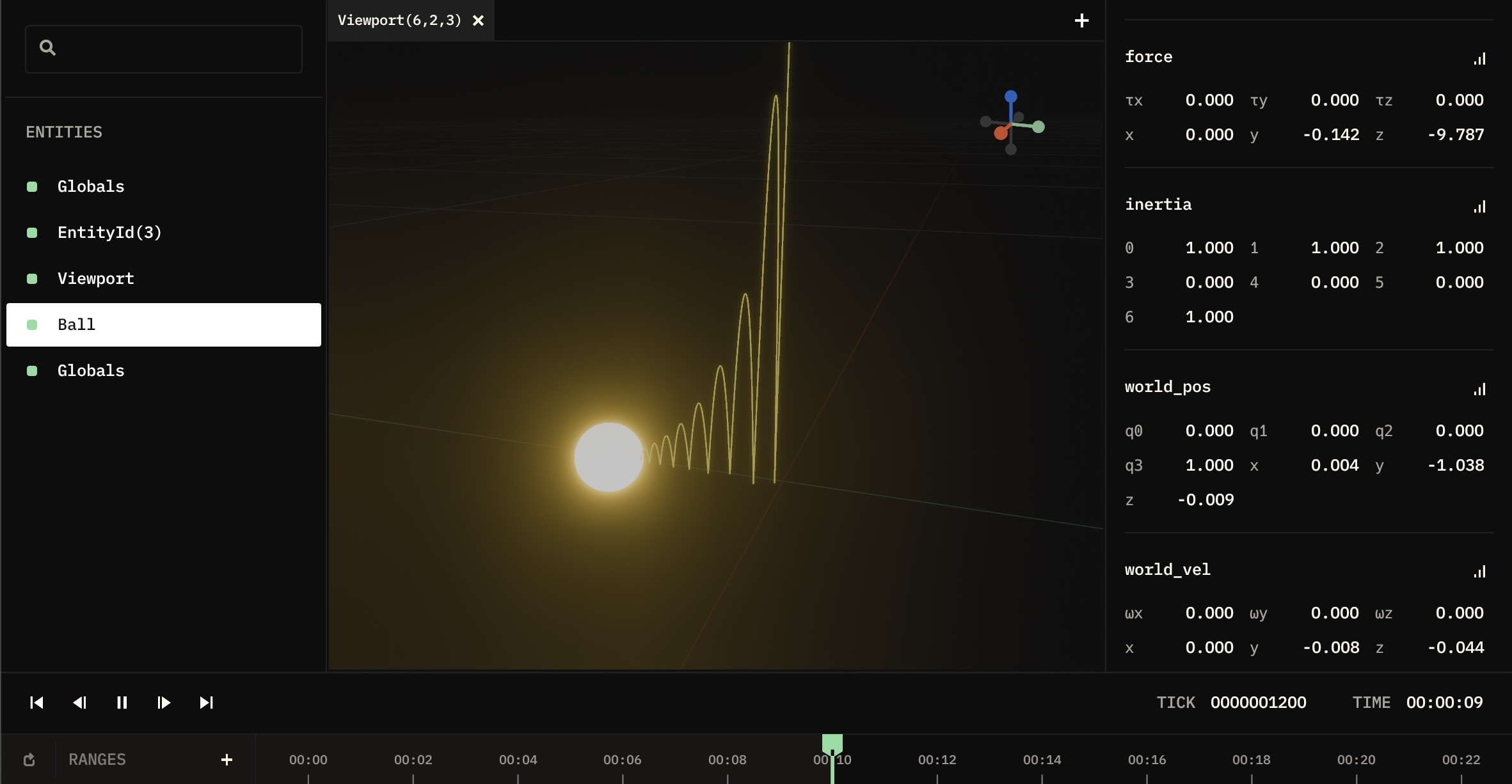
case the simulation only runs for 10 seconds (1200 ticks at 120 ticks per second).
Bouncing off the Ground
You'll notice that the ball falls beautifully, and right through the "ground" into infinity. Let's introduce a system to handle bouncing off the ground instead:
return
The JAX syntax can be visually daunting at first; let's break this down:
The JAX lax.cond function is used to conditionally apply the bounce, if the position of the ball is below the ground.
The first argument is the condition, the second is the function to apply if the condition is true, and the third
is the function to apply if the condition is false. The operand argument is not used in this case, so it's set to None.
Our bounce is applied by reversing the velocity in the z-direction. We'll add "bounciness" later.
Update the System
We now have two systems, gravity and bounce, that we want to apply to our simulation. We can combine them into a single system with the concept of pipelining systems. Let's update our system function:
= |
return
Notice we use a pipe | to combine the systems. This is a powerful concept in Elodin that allows you to chain systems together.
But why is gravity supplied to six_dof, while bounce is not? You'll notice bounce returns the resulting velocity, while gravity only
supplies forces that still need to be applied by an integrator. The six_dof system is an integrator that applies forces to update the
velocity and position of the ball. See the six_dof reference documentation
for more information.
With bounce applied, let's try running it again:
Let's Make it Windy
Having a fully customizable ball bouncing physics simulation is great, but let's make it more interesting by adding some randomized wind forces into the mix. We'll need to make a few changes to our simulation to accommodate this:
Create the Wind Component
We'll need a component to represent the wind force in our simulation:
=
Add Global Wind Data
We'll use a custom Archetype called "WindData" to maintain our random number generator seed and wind state:
: =
: =
Also make sure to update your world function to add a WindData instance:
=
= This is a simple technique to add global data into your simulation for easy reference.

We'll need to set a value for the wind force in our WindData instance. We can do this by creating a system that generates
a random wind force vector and sets it in the Wind component of our WindData instance.
return
This system queries for Archetypes with Seed and Wind components, which will only be our
single "WindData" Archetype entity, and then uses the value of the seed with the random key
function to generate a random wind force vector to set for the Wind component.
Add the Wind Physics System
Now we need a system to apply our wind force to objects. We could just naiively apply the force of the wind
to our ball, but this wouldn't create a physically realistic simulation. Instead we can borrow from
fluid dynamics and leverage the Simple Drag Equation:
$$
F_{d}=c_{d}r\frac{v^2}{2}A
$$
The drag equation states that drag force Fd is equal to the drag coefficient Cd times the density r
times half of the velocity V squared times the reference area A
return 0.5 *
# the Wind entity is a singleton; use the 0th entry of the query result
=
# ball shape generic value (https://en.wikipedia.org/wiki/Drag_coefficient)
= 0.5
# 1.225kg/m^3, density of air at sea level
= 1.225
# magnitude of the wind velocity vector is the scalar fluid velocity value
=
# Area of a hemisphere = 2 * pi * r^2
= 2 * 3.1415 * **2
=
= /
return
return
Let's take a moment to understand @el.system, a lower level API for composing raw systems in Elodin:
When this system is run, it will query for entities with the Wind component and entities with both Force and WorldVel components. These
are provided as arrays of matching entities to the function body as w and q respectively. The function body is then expected to return a
new Query of Force component attached entities, which in this case the Query.map function provides. See
Query.map for more details.
Update the System Function
Finally, we need to update our system function to include the wind and drag systems:
= |
= | |
return
Notice we've made a distinction now of "effectors" as systems which return forces that will be integrated in the 6DoF model.
Improving the Wind Model
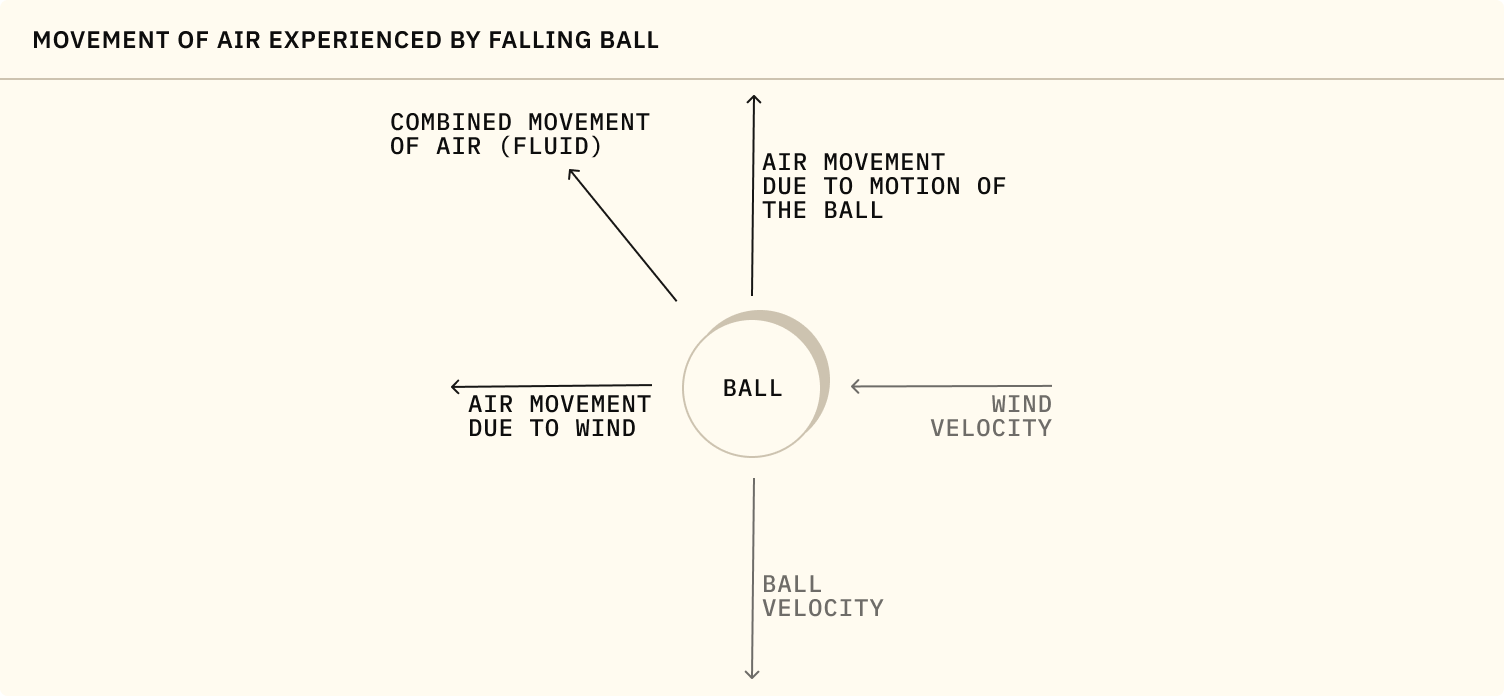
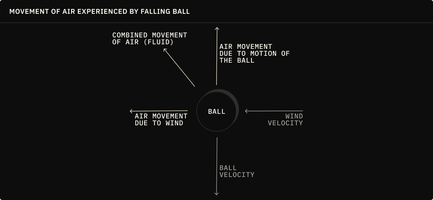
You'll notice that we're currently only considering the velocity of the fluid (wind) in the direction of the wind vector. This is a simplification of the actual drag force due to wind that would be applied to the ball, because the ball's movement through the air also creates a movement of air fluid experienced by the ball.


Let's update our apply_drag system to consider this additional aspect of air fluid movement:
# the Wind entity is a singleton; use the 0th entry of the query result
=
# combine with the ball's velocity to get the relative velocity of fluid movement
-=
...
And voila! We now have a more accurate wind model that accounts for the drag force on the ball as it moves through the air, notice how the ball now loses energy as it struggles against the drag force along it's direction of movement.
Speaking of losing energy, there is one more thing we can do to improve the simulation: Add a coefficient of restitution to represent the "bounciness" of the ball. This will allow us to model the ball losing energy on each bounce.
= 0.85
return
This bounce system uses a coefficient of restitution of 0.85, meaning the ball will lose 15% of its energy on each bounce.
Make it Windy, Simpler
Crafting a simulation in Elodin allows for approaching a problem in multiple ways. We can simplify our wind simulation
by considering the wind not as a global constant, but instead as a force that affects the ball directly, as experienced from the perspective
of the ball entity. This will allow us to use the same apply_drag system, but using the @el.map decorator instead of @el.system,
allowing for a simpler implementation.
Update the Ball Entity
First remove the global spawn of WindData and instead add a WindData component to the ball entity:
=
# world.spawn(WindData(seed=jnp.int64(seed)), name="WindData")
=
Convert use of @el.System
You can now convert the sample_wind system to use the simpler @el.map decorator:
return
And likewise the apply_drag system can be simplified to directly query the wind component from the ball entity,
resulting in much simpler syntax and conceptual model:
=
-=
= 0.5
= 1.225
=
= 2 * 3.1415 * **2
=
= /
return
You should be able to run the simulation and see the same behavior as before, but with a simpler implementation.
Checking your work
Success! We've added a wind force to our simulation. The ball now bounces around the world with the wind affecting its trajectory, steadily blowing the ball in a single direction, losing energy as it bounces. If you'd like to check your work, you can use the following command to generate the matching template code:
You'll notice that the template code is broken into multiple files, this is meant to serve as an example of how you can organize your code as it grows.
Next Steps
The Tao of Elodin
Learn about the design principles behind Elodin.