Three-Body Orbit

The three-body problem is a classic orbital dynamics situation. You have three bodies, each with significant mass, all interacting gravitationally. This turns out to be a chaotic system, with no general closed-form solution. There are however a few stable configurations of the three-body problem.

In this tutorial, we will model one of the stable configurations from R. A. Broucke's technical report "Period Orbits in the Restricted Three-Body Problem with Earth Moon Masses".

Import Elodin and JAX

Our first step is to import Elodin and Jax into our environment:

import elodin as el
from jax import numpy as jnp
from jax.numpy import linalg as la

SIM_TIME_STEP = 1.0 / 120.0

SIM_TIME_STEP value is the duration of each tick in the simulation.

Add 1st & 2nd Body

Before we can do anything we'll need an instance of a World, and with that we can spawn our first entities:

w = el.World()
mesh = w.insert_asset(el.Mesh.sphere(0.2))
a = w.spawn(
    [
        el.Body(
            world_pos=el.WorldPos(linear=jnp.array([1.0, 0.0, 0.0])),
            world_vel=el.WorldVel(linear=jnp.array([0.0, 1.0, 0.0])),
            inertia=el.Inertia(1.0),
        ),
        el.Shape(mesh, w.insert_asset(el.Material.color(25.3, 18.4, 1.0))),
    ],
    name="A",
)
b = w.spawn(
    [
        el.Body(
            world_pos=el.WorldPos(linear=jnp.array([-1.0, 0.0, 0.0])),
            world_vel=el.WorldVel(linear=jnp.array([0.0, -1.0, 0.0])),
            inertia=el.Inertia(1.0),
        ),
        el.Shape(mesh, w.insert_asset(el.Material.color(10.0, 0.0, 10.0))),
    ],
    name="B",
)

Add a basic system

Let's bring in the simplified earth gravity system we just used in the ball example:

@el.map
def gravity(f: el.Force, inertia: el.Inertia) -> el.Force:
    return f + el.SpatialForce(linear=jnp.array([0.0, 0.0, -9.81]) * inertia.mass())

Let's try running the simulation

But first, let's add a view port so we can observe the world:

w.spawn(
    el.Panel.viewport(
        pos=[0.0, -3.0, 3.0],
        looking_at=[0.0, 0.0, 0.0],
        hdr=True,
    ),
    name="Viewport 1",
)

Now, we're ready to start simulating:

sys = el.six_dof(sys=gravity)
sim = w.run(sys, SIM_TIME_STEP)

At this point you should have a running simulation, with two bodies that simply fall just like the ball example. However we don't want a simulation of basic earth gravity, but instead we want the bodies to interact which each other gravitationally like planetary bodies, so let's update our system for that next.

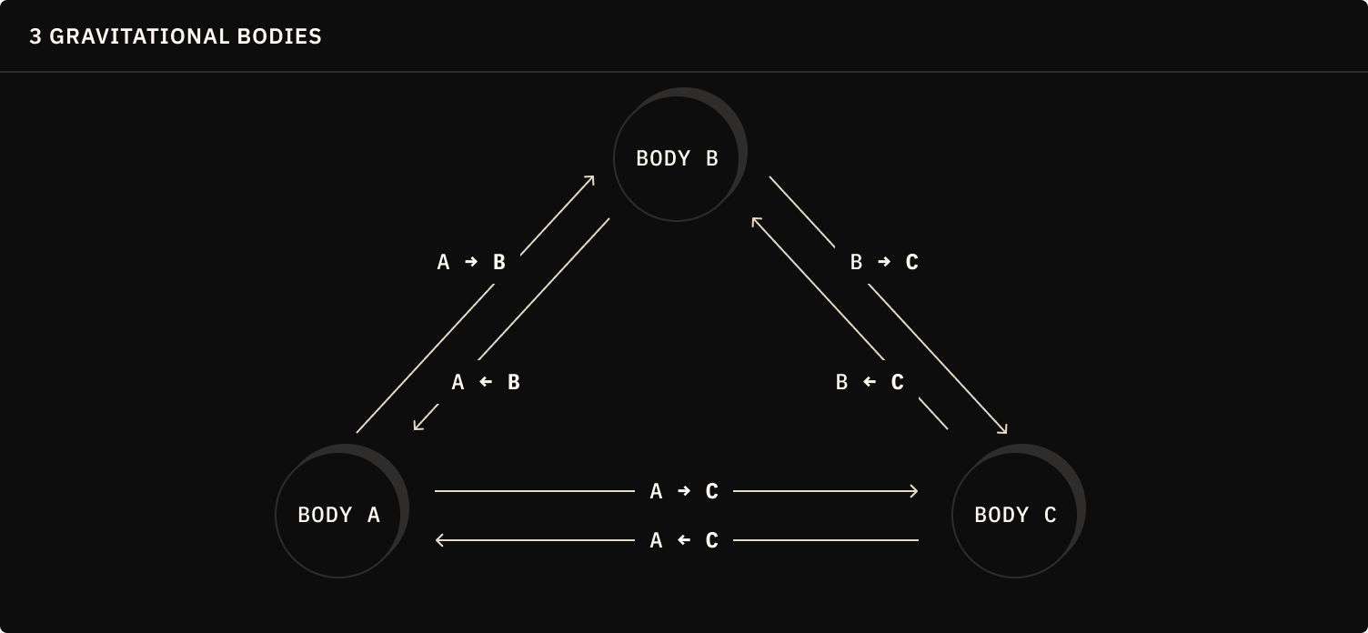
Setup Gravity Constraints

The gravitational force between two bodies is given by Newton's law of universal gravitation: $$ F_{ba}=-G\frac{m_bm_a}{|r_{ba}|^3}{r}_{ba} $$

Notice how we're using the Vector form of Newton's law, instead of the more well known scalar form. This is because we're working in a 3D space. Sometimes you may have to convert between the two forms yourself.

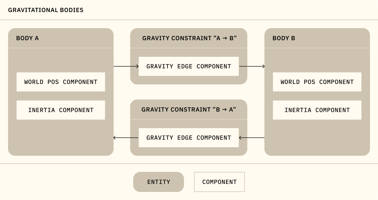
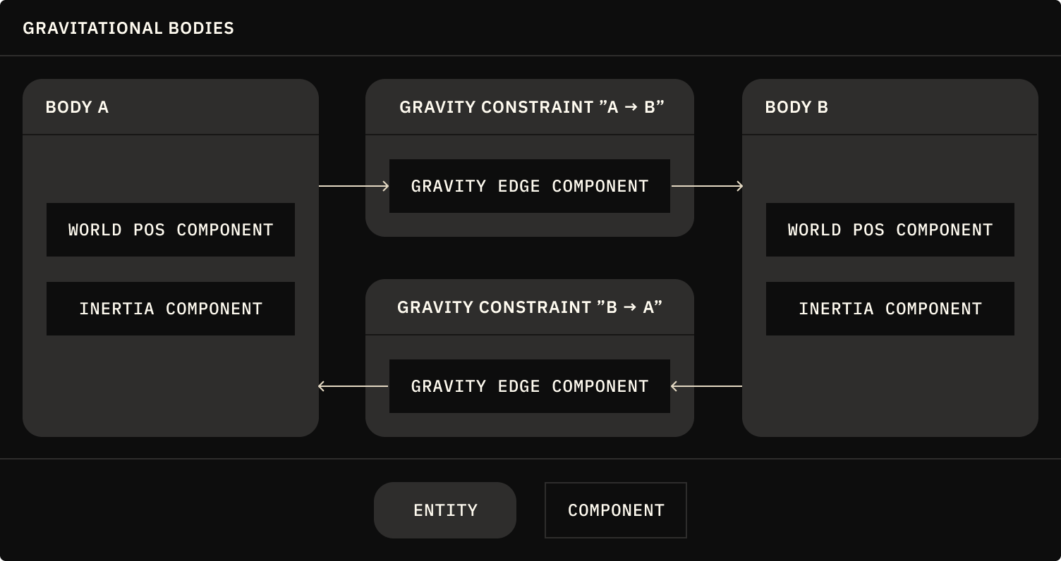
Let's model this as a system that iterates over all gravity edges in a graph of connected bodies and calculates the forces between them. Modeling with graphs and edges is a more advanced Elodin API, review the documentation for it here.

Gravity Constraints Light Gravity Constraints Dark

# Set the gravitational constant for Newton's law of universal gravitation
G = 6.6743e-11

# Define a new "gravity edge" component type
GravityEdge = el.Annotated[el.Edge, el.Component("gravity_edge", el.ComponentType.Edge)]

# Define a new "gravity constraint" archetype using the gravity edge component
@el.dataclass
class GravityConstraint(el.Archetype):
    a: GravityEdge

    def __init__(self, a: el.EntityId, b: el.EntityId):
        self.a = GravityEdge(a, b)

# Replace our simple system with one that applies gravity by iterating over
# all gravity edge components, accessing the positions and inertias of both edges
@el.system
def gravity(
    graph: el.GraphQuery[GravityEdge],
    query: el.Query[el.WorldPos, el.Inertia],
) -> el.Query[el.Force]:
    # Create a fold function to take an accumulator and the query results for the
    # left and right entities, and apply Netwon's law of universal gravitation:
    def gravity_fn(force, a_pos, a_inertia, b_pos, b_inertia):
        r = a_pos.linear() - b_pos.linear()
        m = a_inertia.mass()
        M = b_inertia.mass()
        norm = la.norm(r)
        f = G * M * m * r / (norm * norm * norm)
        # returns the updated force value applied to the left entity this tick
        return el.Force(linear=force.force() - f)

    return graph.edge_fold(
        left_query=query, # i.e. fetches WorldPos and Inertia components from A
        right_query=query, # reusing the same query for B
        return_type=el.Force, # matching the system query return type
        init_value=el.Force(), # initial value for the fold function accumulator
        fold_fn=gravity_fn # the function you defined above to apply to each edge
    )

# Add the gravity constraint entities to the world
w.spawn(GravityConstraint(a, b), name="A -> B")
w.spawn(GravityConstraint(b, a), name="B -> A")

Also let's update the initial mass of our two bodies with the gravitational constant, this will give them a mass more representative of a planetary body:

inertia=el.Inertia(1.0 / G),

Go ahead and run the simulation again, and you should see the two bodies interacting gravitationally.

You'll want to make sure to always keep the six_dof() and w.run() calls at the end of your script.

Add the Third Body

What's a gravitational system without a third body? Let's add a third body to the system.

3-Body Light 3-Body Dark

c = w.spawn(
    [
        el.Body(
            world_pos=el.WorldPos(linear=jnp.array([-0.2, 0, 0])),
            world_vel=el.WorldVel(linear=jnp.array([0, 0.6, 0.0])),
            inertia=el.Inertia(1.0 / G),
        ),
        el.Shape(mesh, w.insert_asset(el.Material.color(0.0, 1.0, 10.0))),
    ],
    name="C",
)

w.spawn(GravityConstraint(a, c), name="A -> C")
w.spawn(GravityConstraint(b, c), name="B -> C")

w.spawn(GravityConstraint(c, a), name="C -> A")
w.spawn(GravityConstraint(c, b), name="C -> B")

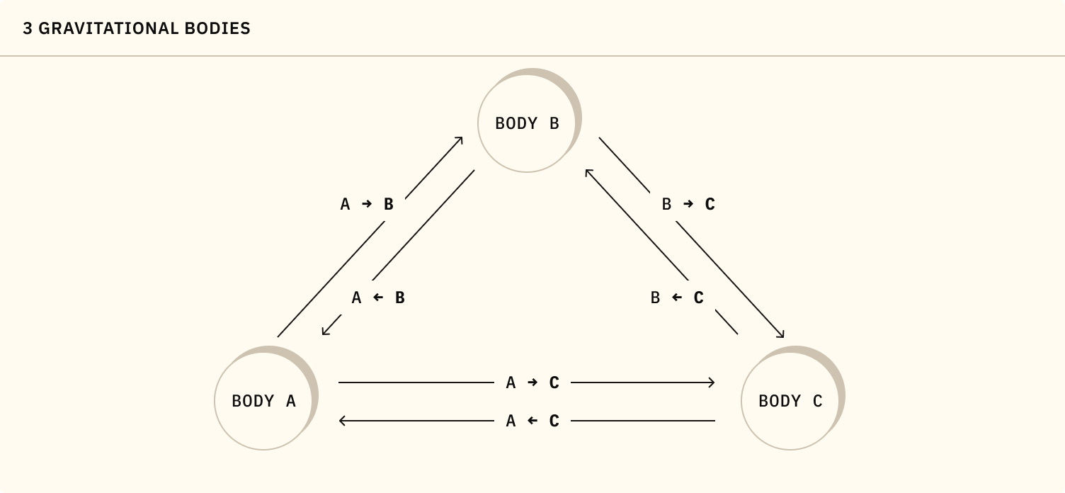
If you run the simulation now, you'll see the three bodies interacting gravitationally. However, you'll notice that the it's a bit unstable.

A stable starting configuration

There are many known stable configurations for three-body systems, one of the most famous being the Lagrange points. For our first attempt we'll reference the Brouke R 7 configuration, which is a stable configuration for three bodies of equal mass.

Go ahead and update the starting values for our three bodies to the following:

a = w.spawn(
    [
        el.Body(
            world_pos=el.WorldPos(linear=jnp.array([0.8920281421, 0.0, 0.0])),
            world_vel=el.WorldVel(linear=jnp.array([0.0, 0.9957939373, 0.0])),
            inertia=el.Inertia(1.0 / G),
        ),
        el.Shape(mesh, w.insert_asset(el.Material.color(25.3, 18.4, 1.0))),
    ],
    name="A",
)
b = w.spawn(
    [
        el.Body(
            world_pos=el.WorldPos(linear=jnp.array([-0.6628498947, 0.0, 0.0])),
            world_vel=el.WorldVel(linear=jnp.array([0.0, -1.6191613336, 0.0])),
            inertia=el.Inertia(1.0 / G),
        ),
        el.Shape(mesh, w.insert_asset(el.Material.color(10.0, 0.0, 10.0))),
    ],
    name="B",
)
c = w.spawn(
    [
        el.Body(
            world_pos=el.WorldPos(linear=jnp.array([-0.2291782474, 0, 0])),
            world_vel=el.WorldVel(linear=jnp.array([0, 0.6233673964, 0.0])),
            inertia=el.Inertia(1.0 / G),
        ),
        el.Shape(mesh, w.insert_asset(el.Material.color(0.0, 1.0, 10.0))),
    ],
    name="C",
)

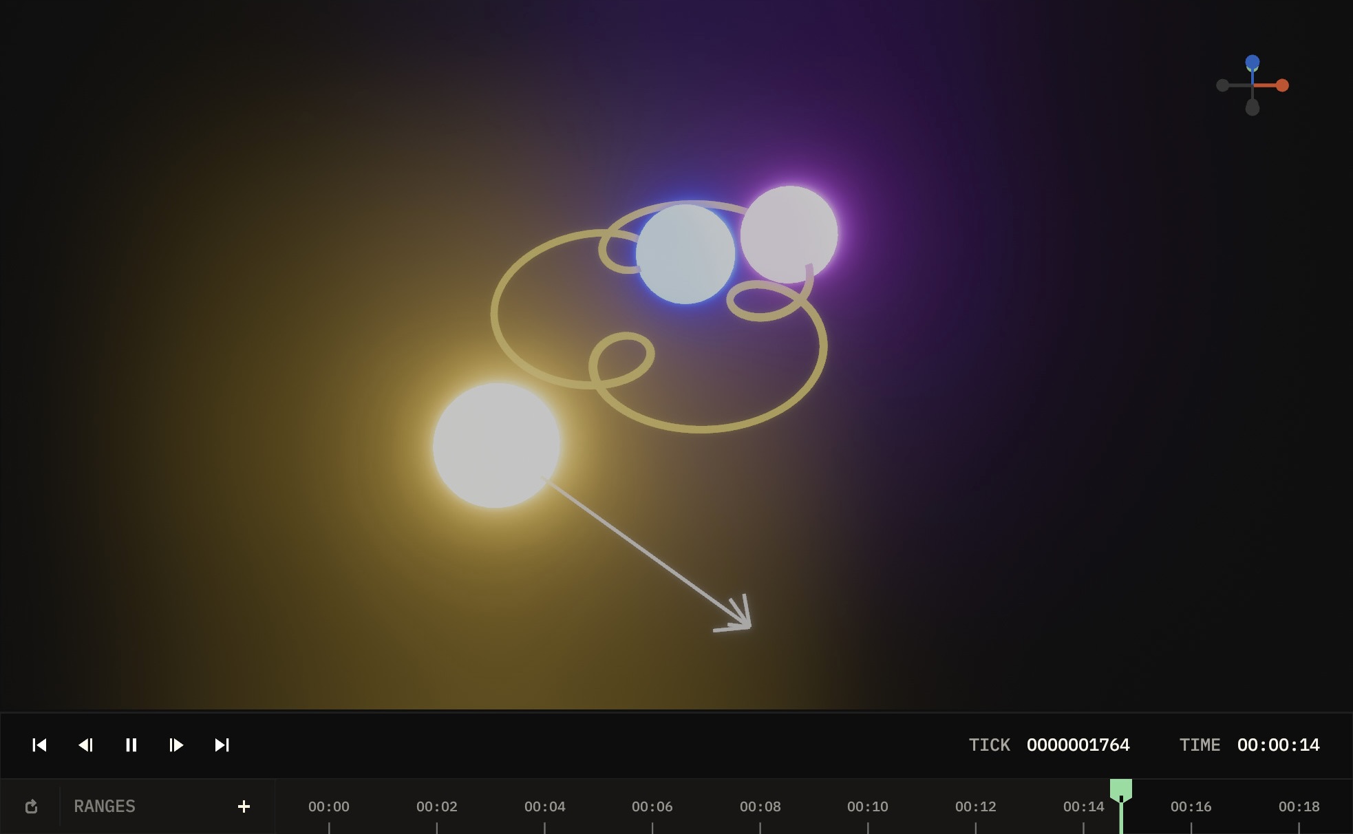
Start the simulation again, and you should see the three bodies in a stable configuration.

Add some gizmos

Sometimes it can be helpful to visualize the forces acting on the bodies and their movements in 3D space. Add these two lines to see a few options in action:

w.spawn(el.VectorArrow(a, "world_vel", offset=3, body_frame=False, scale=1.0))

w.spawn(el.Line3d(b, "world_pos", index=[4, 5, 6], line_width=10.0))

Start the simulation again to see the gizmos in action.

Checking your work

And that's it! You can now run the simulation and see the three bodies orbiting around each other in a stable configuration. If you'd like to check your work, you can use the following command to generate the matching template code:

elodin create --template three-body

Make it fancy

Thanks to the amazing work done here, you can easily try a variety of stable configurations for the three-body system. Let's take the full set of Broucke's stable configurations and randomly select from them on each run of the simulation, for fun.

Add a few new imports to the top of your script, as well as fetching the JSON data from the URL and selecting a random orbit:

import requests
import random
import json

# URL of Bourke's stable orbits JSON data
url = "https://storage.googleapis.com/elodin-assets/brouke-stable-orbits.json"

# Fetch data and select a random orbit
orbit = random.choice(json.loads(requests.get(url).text))

# Example resulting object:
#   {
#     "name": "Broucke A 1",
#     "url": "http://three-body.ipb.ac.rs/bsol.php?id=0",
#     "pos": [
#       [-0.9892620043, 0.0],
#       [2.2096177241, 0.0],
#       [-1.2203557197, 0.0]
#     ],
#     "vel": [
#       [0.0, 1.9169244185],
#       [0.0, 0.1910268738],
#       [0.0, -2.1079512924]
#     ]
#   },

Then update your body creation to use the randomly selected orbit values for each of the three bodies:

The stable orbits are all in the x-y plane, so we set the z element of the position and velocity to 0.0.

a_pos = [float(orbit['pos'][0][0]), float(orbit['pos'][0][1]), 0.0]
a_vel = [float(orbit['vel'][0][0]), float(orbit['vel'][0][1]), 0.0]

b_pos = [float(orbit['pos'][1][0]), float(orbit['pos'][1][1]), 0.0]
b_vel = [float(orbit['vel'][1][0]), float(orbit['vel'][1][1]), 0.0]

c_pos = [float(orbit['pos'][2][0]), float(orbit['pos'][2][1]), 0.0]
c_vel = [float(orbit['vel'][2][0]), float(orbit['vel'][2][1]), 0.0]
a = w.spawn(
    [
        el.Body(
            world_pos=el.WorldPos(linear=jnp.array(a_pos)),
            world_vel=el.WorldVel(linear=jnp.array(a_vel)),
            inertia=el.Inertia(1.0 / G),
        ),
        el.Shape(mesh, w.insert_asset(el.Material.color(25.3, 18.4, 1.0))),
    ],
    name="A",
)
b = w.spawn(
    [
        el.Body(
            world_pos=el.WorldPos(linear=jnp.array(b_pos)),
            world_vel=el.WorldVel(linear=jnp.array(b_vel)),
            inertia=el.Inertia(1.0 / G),
        ),
        el.Shape(mesh, w.insert_asset(el.Material.color(10.0, 0.0, 10.0))),
    ],
    name="B",
)
c = w.spawn(
    [
        el.Body(
            world_pos=el.WorldPos(linear=jnp.array(c_pos)),
            world_vel=el.WorldVel(linear=jnp.array(c_vel)),
            inertia=el.Inertia(1.0 / G),
        ),
        el.Shape(mesh, w.insert_asset(el.Material.color(0.0, 1.0, 10.0))),
    ],
    name="C",
)

And voila, you have a randomly selected stable three-body system!

Going further

You'll notice all of the simulations we've done here are in the x-y plane. As a further exercise, you could try to extend what you've learned here to find and apply the starting configurations for stable three-body systems in all three dimensions.

Post what you discover in the Elodin Discord!

Three-Body Orbit

Import Elodin and JAX

Add 1st & 2nd Body

Add a basic system

Let's try running the simulation

Setup Gravity Constraints

Add the Third Body

A stable starting configuration

Add some gizmos

Checking your work

Make it fancy

Going further

Exploring more bodies